
 |
 |
|
||||||||||
 |


 |
||
multi-Harmony: Sequence Harmony & multi-Relief |
- Synopsis
- Use of the Server
- Multi-group Sequence Harmony
- Multi-Relief
- Empirical significance
- Benchmark
- Bibliography
Read this documentation as formatted PDF.
Synopsis
Many protein families contain sub-families that exhibit functional specialization, which often implies differences in protein-protein interactions. We will present a new interactive web server for the detection of sub-type specific sites, that is easy to use and presents results in a clear and concise way. Results can be analyzed interactively online in a summary table, in the Jalview alignment viewer, and in a Jmol applet using an optional PDB structure. We have generalized the Sequence Harmony method (Pirovano et al., 2006; Feenstra et al., 2007) to handle multiple sub-groups, and also include a deterministic (non sampling) reimplementation of the multi-Relief method (Ye et al., 2008a). The web server, called multi-Harmony, is described, and we compare its performance to other state-of-the-art methods, like SDP-pred (Kalinina et al., 2004b,a) and TreeDet (Carro et al., 2006; Mesa et al., 2003).
This document is also available as formatted PDF.
Other servers
Some other servers that perform similar functions are:
Method Website Reference Sequence Harmony (old) www.ibi.vu.nl/programs/seqharmwww/ Feenstra et al., 2007 Multi-RELIEF (old) www.ibi.vu.nl/programs/multireliefwww/ Ye et al., 2008a PROUST2 www.russell.embl-heidelberg.de/proust2 Hannenhalli and Russell, 2000 ProteinKeys www.proteinkeys.org/proteinkeys Reva et al., 2007 SDPpred bioinf.fbb.msu.ru/SDPpred Kalinina et al., 2004b SDPsite bioinf.fbb.msu.ru/SDPsite Kalinina et al., 2009 TreeDet treedetv2.bioinfo.cnio.es/treedet Carro et al., 2006 Xdet pdg.cnb.uam.es/pazos/mtreedet Pazos et al., 2006
Use of the Server
Input data
The multi-Harmony web server contains main input and advanced options. The main input is a multiple sequence alignment of the protein family and a subdivision into groups. Sanity of the input options is checked, e.g., whether an input alignment is uploaded or pasted, and not both, whether it is a proper alignment format according to one of the supported standards. Problems are reported with an error message and offending input fields are highlighted.
Alignment formats
Your input alignment can be in any of the following supported formats for (aligned) sequences:
FASTA is generally the easiest format to read, write, parse and edit. A simple example is given here:>GROUP:1|Sequence1 DVQAVAYEEPKHWCS >GROUP:1|Sequence2 DAQAVGTEEPKCWCS >GROUP:1|Sequence3 DAQPVATEEPKHWCS >GROUP:2|Sequence4 DLQPVTYCEPAFWCS >GROUP:2|Sequence5 DLQPVAYCEPAFWCS >GROUP:2|Sequence6 DVQPVTYCEPKYWCSGroup definition
Groups can be defined in the sequence labels from the input alignment by including GROUP:# group labels, separated by pipe symbols (|) in the sequence labels, like Q8BGU7_MOUSE |GROUP:1, see also the example given above for Alignment Formats. At minimum, two groups are needed, and each group should have at least two sequences. The order of the labels and sequences is irrelevant; all sequences with identical group labels together form a group.
Alternatively, a set of group sizes can be supplied, in which case the sequences of one group must be contiguous in the alignment, that is, they should be ordered by group. The group sizes can be separated by comma, semicolon, or whitespace. Valid examples of how to represent group sizes for subfamilies are:
All of these examples will be interpreted in the same way: six subfamilies with respective sizes of 3, 2, 5, 6, 10 and 8 sequences.
- 3 2 5 6 10 8
- 3 2 5
6
10 8- 3; 2; 5; 6;
10; 8- 3,2,5 6 10 ; 8
Advanced options
Advanced features allow more control over the analysis and output. A reference sequence can be selected from the alignment to provide a reference numbering in the output tables. Additionally, the selected sites can be visualized in the protein structure using the Jmol applet, if a PDB identifier is specified by its four-letter code, a PDB file uploaded, or retrieved automatically using BLAST. The PDB file is automatically aligned with the multiple alignment, or with the reference sequence if specified. A specific chain of the PDB can be selected, otherwise the chain that best matches the alignment is automatically selected.
Output
The output is a table including all sites, Sequence Harmony scores and multi-Relief weights and associated values, and a summarized view of diversity within and between groups in the so-called ‘Consensus strings’. All numerical columns include toggle buttons for sorting, allowing a fast view of for example the sites with lowest Sequence Harmony scores, or those with highest multi-Relief weights.
The ‘Consensus strings’ columns give all residue types present in each of the groups, respectively. Headers are the group label, either literally from the ’GROUP:’ tags, or an ordinal number when groups were defined by numbers of sequencecs. Appended to the label is the number of sequences in each group in brackets, e.g. like ‘1(9)’. Residue types are sorted in order of decreasing frequency. Residue types that occur with a frequency less than half of the highest are set in lowercase. The Consensus strings columns are hidden by default, and can be displayed by clicking on the ‘Consensus strings’ header.
Sorting and selection of a relevant sites can be done on the numerical columns: Sequence Harmony scores, Z-scores, multi-Relief weights and positive and negative supports. In the sections Sequence Harmony, Empirical Significance and Multi-Relief each of these quantities will be explained in more detail. Sorting on alignment position will recover the sequential ordering of sites.
For Sequence Harmony Z-scores lower is better. The default Z-score cut-off for highlighting is ≤ − 3, but for most datasets a lower Z-score cut-off may be better. The Sequence Harmony cut-off can be between zero (allowing no compositional overlap) and one (allowing full overlap); a higher upper cut-off yields more selected sites.
For multi-Relief weights, support values and Z-scores, higher is better. The multi-Relief cut-off can be between minus one (selecting only ‘locally’ conserved sites) and one (selecting strongly specific sites). A lower bottom cut-off for multi-Relief weights will result in more sites being selected. A good multi-Relief cut-off could be > 0.8, but this may vary with the dataset.
An alternate view of the output data is provided using the Jalview (Clamp et al., 2004) alignment viewer and editor applet. Group definitions are highlighted in the alignment view, and additional rows of annotations are provided for the Sequence Harmony scores (as 1 − SH so high bars are specific sites) and multi-Relief weights. The main page includes a button to transfer selected sites from the table to an annotation track that highlights selected sites. Annotation tracks can be exported from the Jalview applet (use File → Export Annotations...) and for example imported in the full Jalview editor.
If a PDB ID or file was supplied, an optional graphical representations of the selected sites is available as an interactive Jmol applet (Herráez, 2006). In addition, if also a reference sequence was supplied, the PDB structure is passed to Jalview. The Jmol applet includes buttons to highlight sites selected in the output table, and to colour-code residues according to their Sequence Harmony scores or multi-Relief weights. Selections made in the table are dynamically passed to the Jmol applet window.
Implementation
The main steps are as follows. Sequences are read from the alignment and separated into user-specified groups. Sequence Harmony values and multi-Relief weights are calculated as described in the sections Sequence Harmony and multi-Relief. Sequence Harmony values range from zero for completely non-overlapping residue compositions, to one for identical compositions. Multi-Relief values range from one, for highly specific positions, to zero for non-specific positions, to minus one for sites that are variable within groups, but (relatively) conserved globally.
An optional protein structure (PDB file) can be supplied by its PDB ID, by PDB file upload, or by automatic selection using BLAST (Altschul et al., 1997). The selected chain from the PDB structure will be aligned with the selected reference sequence using the ‘profile’ option of MUSCLE (Edgar, 2004). If no PDB chain was supplied by the user, all individual chains will be aligned in turn. Subsequently the chain is selected that has the shortest hamming distance (is most similar) to the reference sequence. If no reference sequence was selected, the PDB chain will be profile-aligned with the whole input alignment. In the case that also no PDB chain was selected, the chain with the shortest hamming distance to any sequence in alignment is selected. The resulting alignment between PDB chain and alignment is used to map selected sites in the output to the PDB structure.
BLAST is carried out against the non-redundant PDB protein sequence database without low-complexity filtering, an E-value threshold of 10−3 and otherwise default options (details are available in the BLAST report in the Download section of the results). Although we provide this option for convenience, we advise users to select a good PDB sequence themselves.
Sorting and selection is implemented in JavaScript in the output table. Selections are dynamically passed to the optional Jmol window for display in the protein structure. In addition, selections can be added as annotations in the Jalview alignment window. Currently alignments of up to about two thousand sequences can be processed with a runtime in the order of minutes.
Multi-group Sequence Harmony
Pairwise Sequence Harmony
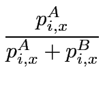
The Sequence Harmony method, as described previously (Pirovano et al., 2006), finds specificity-determining residues from pair-wise comparison of functional groups of protein sequences. The algorithm is implemented as a python program. Sequences are taken from the alignment and separated into user-specified groups. Sequence Harmony values are calculated from a form of mutual information using the sum of the normalised frequencies of groups A and B:
for position i in the alignment, and a sum over residue types x. In addition, we take the average of SHA/AB and SHB/AB to obtain symmetrical score values:
Sequence Harmony values range from zero for completely non-overlapping residue compositions, to one for identical compositions.
Note that SHpair from Eqn. 2 can equivalently be expressed as the difference between the total entropy and the sum of group entropies, as explained in Pirovano et al., 2006 and Feenstra et al., 2007. This is reminiscent of the ‘Two-entropies analysis’ of Ye et al., 2008b, except that in the Sequence Harmony formulation the total entropy is calculated weighing each group equally, instead of each sequence.
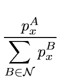
Multi-group as General Sum in Probabilities
Potentially there are several ways to generalize Eqn. 1 for multiple (N > 2) groups, that work out to give slightly different weightings to different sites. A straightforward generalization over a set
of N groups, is to generalize the sum pA + pB (Eqn. 1), as follows
and the average over all SHA/
, cf. Eqn. 2, as
Since this formulation is expressed in amino acid frequencies p (probabilities), we refer to this generalization as ‘Frequency’: SHFreq.
Shannon’s Alphabet Size
We retain the bounded behaviour of this score on the [0...1] interval, cf. Eqn. 2, by using Shannon’s ‘alphabet size’ as the base of the logarithms. We get the base as b = min(NAA, Nseq) for an amino acid alphabet size of NAA and Nseq sequences in a group. (This has confusingly been referred to as ‘scaled logarithm’, e.g. by Ye et al., 2008b.) With this, the entropies and therefore SHFreq run on the interval [0...1]. It should be noted that the effect is not just a scaling of values, which would nevertheless be convenient for defining a general cut-off scheme, but also the ranking of sites is affected due to a change in the balance between the terms.
Multi-Relief
The multi-Relief method, as introduced previously (Ye et al., 2008a), finds specificity-determining residues using the multi-Relief algorithm and functional groups of in the input alignment. This algorithm has been reimplemented as a python program. Sequences are taken from the alignment and separated into user-specified groups. Multi-Relief weights are calculated from application of the Relief algorithm to pairs of groups in the input alignment. Completely conserved positions and overall divergent positions will get zero weight, while positions that are divergent within subfamilies but conserved between subfamilies will get negative weight. If a residue position is conserved within each group but divergent between groups, then its Relief weight will be high.
Deterministic versus Sampled
In the original implementation (Ye et al., 2008a) a random sampled sub-set of pairs of groups at the multi-Relief step (iterations), and of sequences within groups at the (pairwise) Relief step (sample size), was used on the assumption that this results in an efficient calculation without sacrifice of accuracy. This was based on the observation that calculated weights converged rapidly with increased iterations and sample size.
Detailed analysis of several additional datasets revealed the possibility of calculation artefacts introduced by the random sub-sampling. Additional performance benchmarks on deterministic code that explicitly calculates all possible pairs of groups and all sequences showed that large datasets could still be processed in reasonable calculation time (several minutes for the GPCR dataset with 2000 sequences and 77 groups). Furthermore, it was realized that the ‘nearest hit’ and ‘nearest miss’ that are used in the Relief algorithm are not necessarily unique; due to the presence of identical distances between sequences, multiple hits could be retrieved. Therefore, an additional loop over all combinations of nearest hits and nearest misses was added. This resulted in the following elaborated pseudo-code:
multiRelief ( groups ):
""" compare all groups with each other to calculate the Relief and
matrix scores, expects a list of groups objects as input """
total_weights_list = zero list
# perform Relief for all pairs of groups:
for groupA , groupB in unique pairs of groups :
total_weights_list += Relief ( groupA , groupB )
# calculate average weights
for each alignment position i :
if positive weights at i :
weights [ i ] = average ( positive weights at i )
else:
if negative weights at i :
weights [ i ] = average (negative weights at i )
else:
# if no negative or positive weights, it must be zero:
weights [ i ] = 0
return weights
Given sequences from two groups, Relief assigns weights to features based on how well they separate samples from their nearest neighbours (nnb) from the same and from the opposite group (Marchiori et al., 2006). Relief incrementally updates a weight vector. At each iteration, one sequence seq is selected. The weights are updated by adding the ‘difference’ between seq and its nnb from the opposite group, miss(seq), and subtracting the difference between seq and its nnb from the same group, hit(seq). We define nnb for a sequence seq to group ‘A’ as nnb(seq) = argmin{d (seq, x) x ∈ groupA} where d denotes the Hamming distance between strings (e.g., d (ALM,VLM) = 1). The difference between two sequences seq1 − seq2 is a vector representing matches (0) and mismatches (1) between residues (e.g., ALM − VLM = 100). This procedure is iterated over all sequences of the dataset. The computational complexity of Relief is O(nr_ seq2 . nr_ positions).
Relief ( groupA , groupB ):
""" calculate the weights of this group compared to the
sequences in this group and add those weights to the
weights in this group """
total_weights = zero list
for sequence in groupA , groupB :
this_group = group A or B where sequence resides
other_group = not this_group
for sequence in this_group :
nearest_hits = Nearest Neighbour(s) of sequence in this_group
nearest_misses = Nearest Neighbour(s) of sequence in other_group
weights = zero list
# we can have multiple nearest hits/misses (identical distances):
for hit_sequence in nearest_hits :
for mis_sequence in nearest_misses :
mis_diff = sequence − mis_sequence # sequence difference
hit_diff = sequence − hit_sequence # sequence difference
weights += mis_diff − hit_diff # bit-vector difference
# normalize over combinations of nearest hits and misses:
weights /= len ( nearest_hits ) * len ( nearest_miss )
total_weights_this += weights
# normalize over sequences in this group:
total_weights_this /= len ( this_group )
total_weights += total_weights_this
# normalize over forward and backward comparison:
total_weights /= 2
return total_weights
Support values for positive and negative weights are also reported by multi-Relief, in addition to the weight values that are used for ranking specificity sites. The support is expressed as the fraction of positive, respectively negative, weight values obtained from Relief for all pairs of groups.
Empirical significance
In addition to the scores that will be used for ranking specificity sites, a significance estimate is performed to allow for the selection of reliably ranked sites only. This reliability is expressed as empirical Z-scores over a set of Sequence Harmony and multi-Relief values obtained from permutations (randomized groupings) over the input alignment.
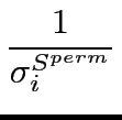
Z-scores give a measure of how far the observed score, either Sequence Harmony value or multi-Relief weight, deviates from the mean of the distribution obtained from randomized scores. Z-scores are calculated as:
with
...
expressing the average, σSperm = √
( Sperm −
Sperm
)2
the standard deviation over Sperm, and Sperm the set of scores obtained from the random permuations. For completely conserved positions, the standard deviation σ is zero, and the Z-score is therefore undefined. This is denoted as ‘nan’ (not a number) in the output table. For Sequence Harmony, low scores are the important ones, a lower (negative) Z-score indicates highly significant specificity positions. For multi-Relief it is high scores, and therefore high (positive) Z-scores that indicate significant specificity.
Benchmark
We compare the Sequence Harmony and multi-Relief results with other algorithms included in our previous work, using the same datasets (Pirovano et al., 2006; Ye et al., 2008a). Default parameter settings for all algorithms were used. For constructing the plots of Precision TP/(TP+FP) vs. Recall TP/(TP+FN), ranked lists of sites for Sequence Harmony, multi-Relief and SDP-pred were used, and for TreeDet/MB the cut-off value was varied from 0 to 1.0. Definitions of true positive sites, as well as TP, FP and FN, are used from Pirovano et al., 2006 and Ye et al., 2008a.
Table 1: Benchmark scores for detection of specificity sites by five methods as area-under-curve (AUC) for the Precision/Revall plots versus gold-standard specificity sites, for 22 datasets. Best-scoring methods for each dataset are set in bold. Averages per method and per datset, and standard deviation per method are also reported.
Dataset Nr. multi- mR Sequence SH SDP Xdet Xdet PROU Protein Average Pos. Relief Z< 6 Harmony Z< − 9 pred supervised ST2 Keys cbm9 7 0.161 0.161 0.074 0.074 0.122 0.352 0.209 0.349 0.049 0.352 cd00120 3 0.058 0.058 0.054 0.054 0.126 0.106 0.106 0.079 0.008 0.126 cd00264 3 0.006 0.006 0.003 0.003 0.017 0.080 0.019 0.012 0.087 0.087 cd00333 12 0.301 0.301 0.287 0.287 0.376 0.366 0.346 0.055 0.203 0.376 cd00363 6 0.010 0.010 0.008 0.008 0.012 0.009 0.012 0.009 0.010 0.012 cd00365 10 0.055 0.055 0.119 0.119 0.126 0.103 0.189 0.016 0.010 0.189 cd00423 4 0.204 0.204 0.080 0.080 0.234 0.196 0.171 0.049 0.002 0.234 cd00985 3 0.329 0.329 0.198 0.198 0.509 0.387 0.534 0.058 0.034 0.534 CNmyc 11 0.037 0.037 0.067 0.067 0.187 0.086 0.101 0.122 0.027 0.187 GPCR190 21 0.246 0.252 0.486 0.517 0.508 0.125 0.275 0.308 0.377 0.517 GPCR 21 0.347 0.347 0.489 0.489 0.583 − * − * − * 0.505 0.583 GST 9 0.156 0.156 0.242 0.242 0.615 0.117 0.402 0.446 0.483 0.615 IDH_IMDH 14 0.050 0.050 0.048 0.048 0.196 0.100 0.129 0.089 0.065 0.196 LacI 28 0.266 0.282 0.124 0.207 0.146 0.188 0.207 0.098 0.301 0.301 MDH_LDH 1 0.063 0.063 0.125 0.125 0.250 0.033 0.250 0.015 0.005 0.250 MIP 23 0.213 0.216 0.249 0.268 0.242 0.169 0.208 0.187 0.119 0.268 nucl. cycl. 2 0.417 0.417 0.413 0.413 0.413 0.054 0.292 0.305 0.011 0.417 rab5+6 28 0.540 0.539 0.602 0.602 0.416 0.322 0.346 0.455 0.364 0.602 ras+ral 12 0.666 0.666 0.540 0.540 0.357 0.398 0.545 0.378 0.092 0.666 ricin 21 0.186 0.186 0.194 0.194 0.201 0.173 0.193 0.256 0.276 0.276 serine 2 0.078 0.078 0.261 0.261 0.542 0.105 0.750 0.750 0.006 0.750 Smad 29 0.719 0.721 0.713 0.703 0.522 0.686 0.677 0.721 0.748 0.748 Average 12 0.232 0.233 0.244 0.250 0.305 0.198 0.284 0.226 0.172 0.305 Std Dev 0.205 0.205 0.208 0.207 0.187 0.164 0.201 0.225 0.209 0.225
Bibliography
- Altschul, S. F., Madden, T. L., Schaffer, A. A., Zhang, J., Zhang, Z., Miller, W., and Lipman, D. J. (1997).
- Gapped blast and psi-blast: a new generation of protein database search programs.
Nucl. Acids Res., 25:3389−3402.
http://blast.ncbi.nlm.nih.gov.
- Carro, A., Tress, M., de Juan, D., Pazos, F., Lopez-Romero, P., Del Sol, A., Valencia, A., and Rojas, A. (2006).
- TreeDet: a web server to explore sequence space.
Nucl. Acids Res., 35(Web Server Issue):99.
http://treedetv2.bioinfo.cnio.es/treedet/.
- Clamp, M., Cuff, J., Searle, S. M., and Barton, G. J. (2004).
- The Jalview Java alignment editor.
Bioinf., 20(3):426−7.
http://www.jalview.org.
- Edgar, R. C. (2004).
- MUSCLE: multiple sequence alignment with high accuracy and high throughput.
Nucl. Acids Res., 32(5):1792−7.
- Feenstra, K., Pirovano, W., Krab, K., and Heringa, J. (2007).
- Sequence harmony: detecting functional specificity from alignments.
Nucl. Acids Res., 35(web server issue):W495-W498.
http://www.ibi.vu.nl/programs/seqharmwww/.
- Hannenhalli, S. S. and Russell, R. B. (2000).
- Analysis and prediction of functional sub-types from protein sequence alignments.
J. Mol. Biol., 303(1):61−76.
http://www.russell.embl-heidelberg.de/proust2.
- Herráez, A. (2006).
- Biomolecules in the computer: Jmol to the rescue.
Biochem. Educ., 34:255−261.
http://www.jmol.org.
- Kalinina, O., Gelfand, M., and Russell, R. (2009).
- Combining specificity determining and conserved residues improves functional site prediction.
BMC Bioinformatics, 10:174.
http://bioinf.fbb.msu.ru/SDPsite/.
- Kalinina, O. V., Mironov, A. A., Gelfand, M. S., and Rakhmaninova, A. B. (2004a).
- Automated selection of positions determining functional specificity of proteins by comparative analysis of orthologous groups in protein families.
Prot. Sci., 13(2):443−56.
- Kalinina, O. V., Novichkov, P. S., Mironov, A. A., Gelfand, M. S., and Rakhmaninova, A. B. (2004b).
- SDPpred: a tool for prediction of amino acid residues that determine differences in functional specificity of homologous proteins.
Nucl. Acids Res., 32(Web Server issue):W424−8.
http://bioinf.fbb.msu.ru/SDPpred/.
- Marchiori, E., Pirovano, W., Heringa, J., and Feenstra, K. (2006).
- A feature selection algorithm for detecting subtype specific functional sites from protein sequences for smad receptor binding.
In Fifth International Conference on Machine Learning and Applications, pages 168−173. IEEE.
- Mesa, A. D. S., Pazos, F., and Valencia, A. (2003).
- Automatic methods for predicting functionally important residues.
J. Mol. Biol., 326(4):1289−1302.
- Pazos, F., Rausell, A., and Valencia, A. (2006).
- Phylogeny-independent detection of functional residues.
Bioinformatics, 22:1440−8.
http://pdg.cnb.uam.es/pazos/mtreedet.
- Pirovano, W., Feenstra, K. A., and Heringa, J. (2006).
- Sequence comparison by sequence harmony identifies subtype specific functional sites.
Nucl. Acids Res., 34(22):6540−6548.
- Reva, B., Antipin, Y., and Sander, C. (2007).
- Determinants of protein function revealed by combinatorial entropy optimization.
Genome Biol., 8:R232.
http://www.proteinkeys.org/proteinkeys.
- Ye, K., Feenstra, K. A., Heringa, J., IJzerman, A. P., and Marchiori, E. (2008a).
- Multi-relief: a method to recognize specificity determining residues from multiple sequence alignments using a machine learning approach for feature weighting.
Bioinf., 24:18−25.
http://www.ibi.vu.nl/programs/multireliefwww/.
- Ye, K., Vriend, G., and IJzerman, A. P. (2008b).
- Tracing evolutionary pressure.
Bioinf., 24:908−915.
http://entropy.liacs.nl/.
(c) IBIVU 2024. If you are experiencing problems with the site, please contact the webmaster.